Vertical and Horizontal Integration Tutorial for ST and SM Data

cd ..

/home/rolan/Documents/spatialMETA

/home/rolan/miniconda3/envs/spatialtk/lib/python3.9/site-packages/IPython/core/magics/osm.py:417: UserWarning: using dhist requires you to install the `pickleshare` library.
  self.shell.db['dhist'] = compress_dhist(dhist)[-100:]

This tutorial demonstrates the process of vertically and horizontally integrating aligned and reassigned ST and SM data using spatialMETA. Vertical and horizontal integration is a powerful technique to address modality fusion and batch effects.

import spatialmeta as smt
import numpy as np
import pandas as pd
import scanpy as sc
import torch
import copy
import matplotlib.pyplot as plt

RCC_sample_list = ["R114_T","S15_T","X49_T","Y27_T","Y7_T"]

Read and preprocess data

Read and merge data

In this step, we read and merge data.

# If data is available
for i in ["R114_T","S15_T","X49_T","Y27_T","Y7_T"]:
    joint_adata = sc.read_h5ad("./adata_joint_"+i+"_raw.h5ad")
    joint_adata_name = "joint_adata_" +i
    globals()[joint_adata_name] = joint_adata

#Test data can be obtained from SpatialMETA
for i in ["R114_T","S15_T","X49_T","Y27_T","Y7_T"]:
    joint_adata = smt.data.load_adata(
        sample_name= i+"_raw",
        modality="joint"
    )
    joint_adata_name = "joint_adata_" +i
    globals()[joint_adata_name] = joint_adata

merge_adata = anndata.concat({
"R114_T":joint_adata_R114_T,
"S15_T":joint_adata_S15_T,
"X49_T":joint_adata_X49_T,
"Y27_T":joint_adata_Y27_T,
"Y7_T":joint_adata_Y7_T,
},label="sample")

/home/rolan/miniconda3/envs/spatialtk/lib/python3.9/site-packages/anndata/_core/anndata.py:1828: UserWarning: Observation names are not unique. To make them unique, call `.obs_names_make_unique`.
  utils.warn_names_duplicates("obs")

merge_adata.var = joint_adata_Y7_T.var

merge_adata

AnnData object with n_obs × n_vars = 20038 × 37703
    obs: 'x_coord', 'y_coord', 'spot_name', 'total_intensity', 'mean_intensity', 'n_genes_by_counts', 'log1p_n_genes_by_counts', 'total_counts', 'log1p_total_counts', 'pct_counts_in_top_50_genes', 'pct_counts_in_top_100_genes', 'pct_counts_in_top_200_genes', 'pct_counts_in_top_500_genes', 'total_counts_mt', 'log1p_total_counts_mt', 'pct_counts_mt', 'n_counts', 'sample'
    var: 'name', 'type'
    obsm: 'spatial'

Normalize merge data

In this step, we normalize the merged data.

merge_adata.layers["counts"] = merge_adata.X.copy()

smt.pp.normalize_total_joint_adata_sm_st(merge_adata,
                         target_sum_SM=1e4,
                         target_sum_ST=1e4)

merge_adata.layers["normalized"] = merge_adata.X.copy()

Quality control

We perform quality control to remove low-quality spots.

merge_adata = merge_adata[merge_adata.obs['total_intensity']>=1e5]

merge_adata = merge_adata[merge_adata.obs['total_counts']<=40000]

Calculate SVGs/SVMs and remove batch-baised SVGs/SVMs

We also calculate spatial variable genes/metabolites(SVGs/SVMs) to identify features that exhibit spatial variation. In addition, we remove those that are batch-biased.

smt.pp.spatial_variable_joint_adata_sm_st(
    merge_adata,
    n_top_genes = 2500,
    n_top_metabolites = 1000,
    batch_key="sample",
    min_samples = 3,
    min_frac = 0.9,
    min_logfc= 3,
)

WARNING: It seems you use rank_genes_groups on the raw count data. Please logarithmize your data before calling rank_genes_groups.

merge_data = merge_adata[:,merge_adata.var.highly_variable_moranI]

merge_data

View of AnnData object with n_obs × n_vars = 19860 × 2841
    obs: 'x_coord', 'y_coord', 'spot_name', 'total_intensity', 'mean_intensity', 'n_genes_by_counts', 'log1p_n_genes_by_counts', 'total_counts', 'log1p_total_counts', 'pct_counts_in_top_50_genes', 'pct_counts_in_top_100_genes', 'pct_counts_in_top_200_genes', 'pct_counts_in_top_500_genes', 'total_counts_mt', 'log1p_total_counts_mt', 'pct_counts_mt', 'n_counts', 'sample'
    var: 'name', 'type', 'highly_variable_moranI'
    obsm: 'spatial'
    layers: 'counts', 'normalized'

merge_adata.write_h5ad("./spatialmeta_tutorial/data/ccRCC_merge_hvf.h5ad")

ConditionalVAE for horizontal integration for ST and SM

In this step, we perform horizontal integration using the ConditionalVAE model.

merge_adata.X = merge_adata.layers["counts"]

smt.pp.normalize_total_joint_adata_sm_st(
    merge_adata,
    target_sum_SM=1e3,
    target_sum_ST=None
)

model = smt.model.ConditionalVAESTSM(
    merge_adata,
    n_latent=10,
    device='cuda:0',
    batch_keys= ["sample"],
    batch_embedding="embedding",
    reconstruction_method_sm='g',
    reconstruction_method_st='zinb',
)

loss_dict = model.fit(
    max_epoch=64,
    lr=1e-3,
    kl_loss_reduction= 'mean',
    mode='multi'
)

/home/rolan/Documents/spatialMETA/spatialmeta/util/logger.py:151: TqdmWarning: IProgress not found. Please update jupyter and ipywidgets. See https://ipywidgets.readthedocs.io/en/stable/user_install.html
  from tqdm.autonotebook import tqdm as tqdm_notebook
Epoch 64: 100%|██████████| 64/64 [05:15<00:00,  4.93s/it, reconst_sm=-2.29e+03, reconst_st=5.86e+03,

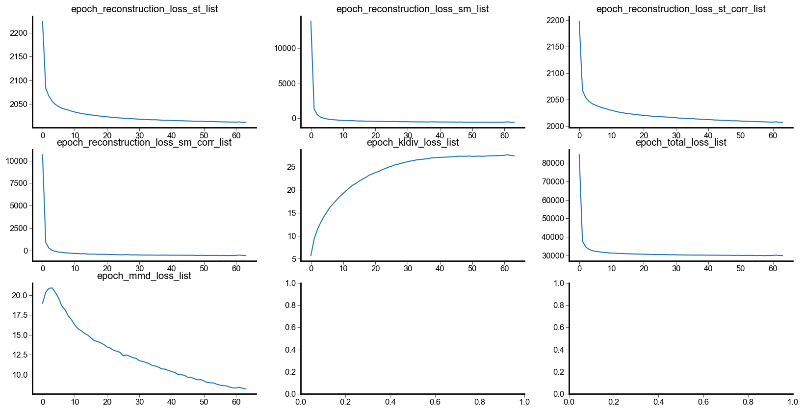
Loss visualization

fig,axes=createSubplots(3,3,figsize=(20,10))
axes=axes.flatten()
for ax,(k,v) in zip(axes, loss_dict.items()):
    ax.plot(v)
    ax.set_title(k)

Visualization and analysis

Z = model.get_latent_embedding()
X = model.get_normalized_expression()
C = model.get_modality_contribution()

Latent Embedding: 100%|██████████| 156/156 [00:00<00:00, 161.02it/s]
Latent Embedding: 100%|██████████| 156/156 [00:04<00:00, 32.68it/s]
Latent Embedding: 100%|██████████| 156/156 [00:00<00:00, 161.32it/s]

merge_adata.layers['reconstruction'] = X
merge_adata.obsm['X_emb']=Z
merge_adata.obs['contribution_st']=C
merge_adata.obs['contribution_sm']=1-C

sc.pp.neighbors(merge_adata,
                use_rep="X_emb",
                n_neighbors=20)

sc.tl.umap(merge_adata,
           min_dist=1,
           spread=1)

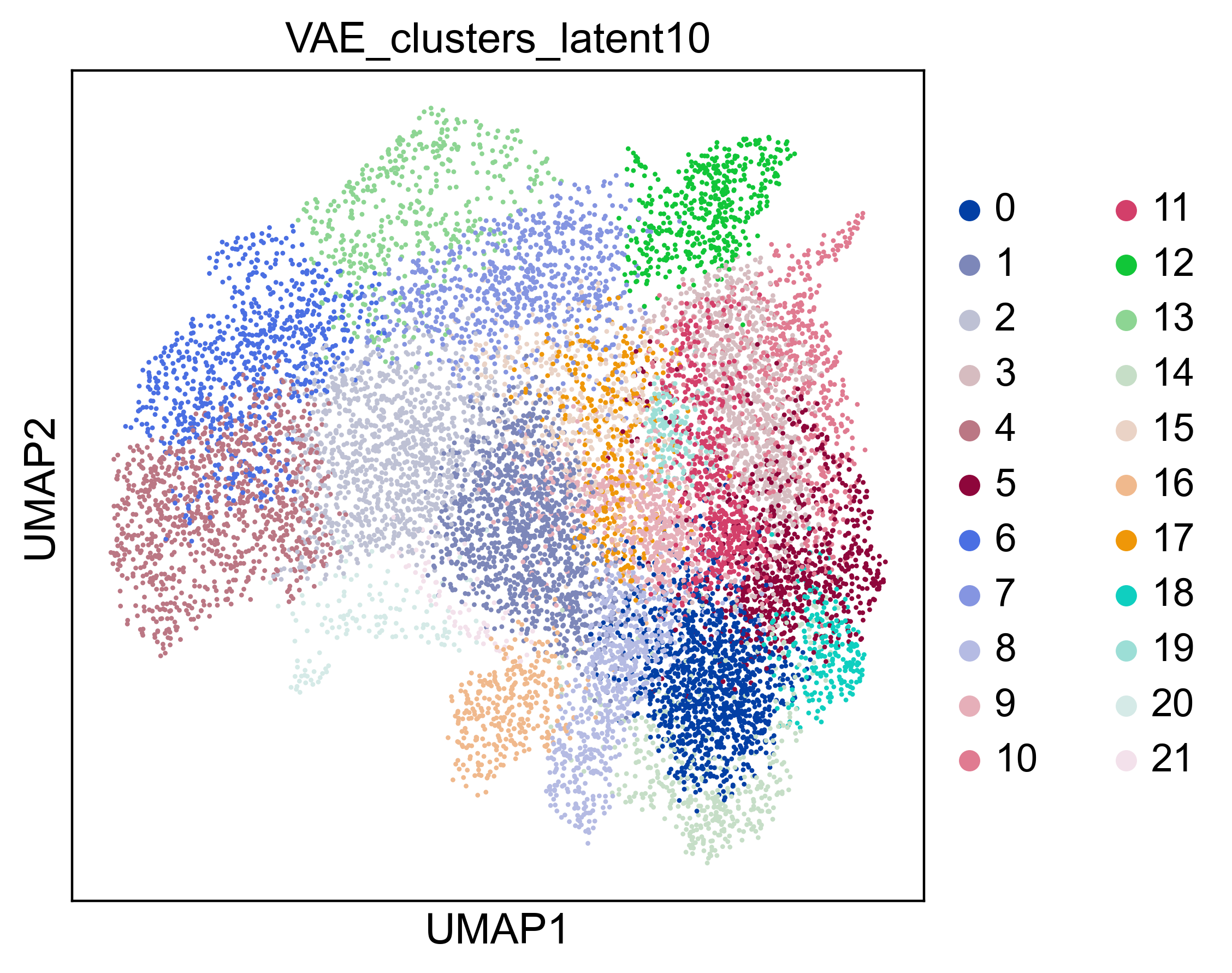
sc.tl.leiden(merge_adata,
             resolution= 1,
             key_added="VAE_clusters_latent10")

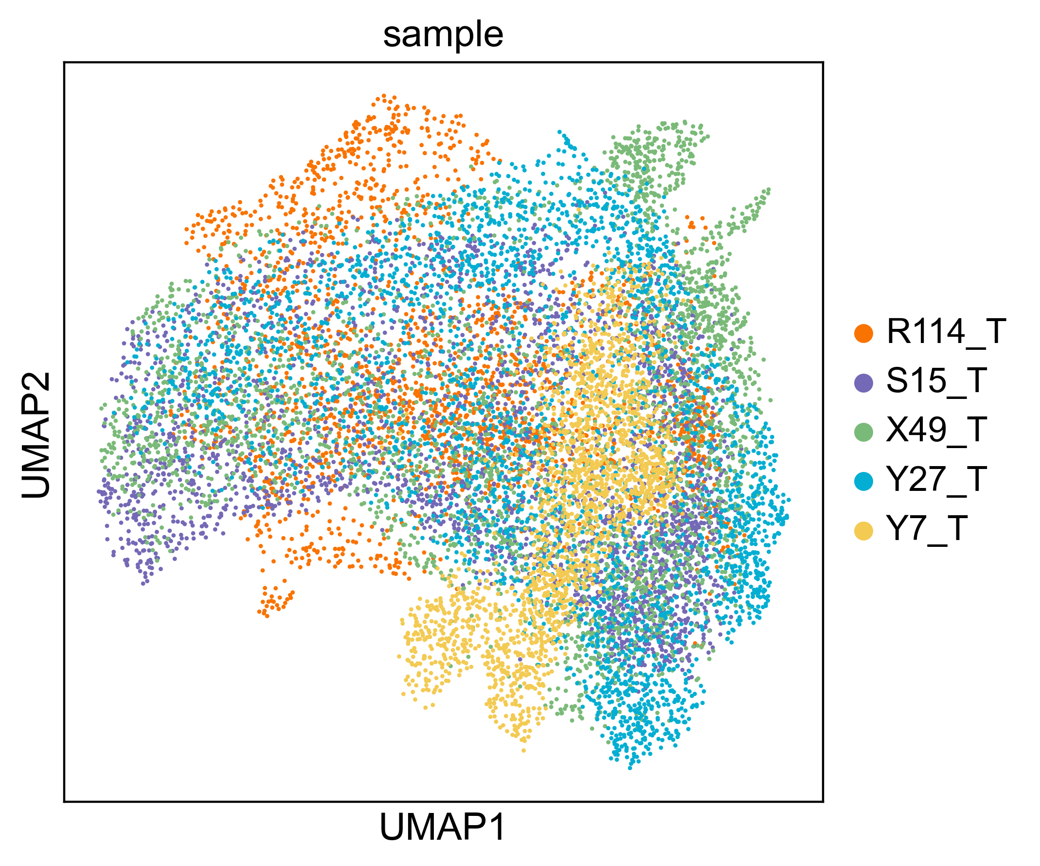
sc.settings.set_figure_params(dpi=200, facecolor="white")
fig,ax=plt.subplots()
fig.set_size_inches(5,5)
sc.pl.umap(merge_adata,
           color=["sample"],
           palette = {
              "R114_T": "#F97300",
              "S15_T": "#7469B6",
              "X49_T": "#7ABA78",
              "Y27_T": "#03AED2",
              "Y7_T": "#F3CA52",
           },
           show = False,
           size = 10,
           ax=ax
)

<Axes: title={'center': 'sample'}, xlabel='UMAP1', ylabel='UMAP2'>

sc.settings.set_figure_params(dpi=200, facecolor="white")
fig,ax=plt.subplots()
fig.set_size_inches(5,5)
sc.pl.umap(merge_adata,
           color=["VAE_clusters_latent10"],
           palette = sc.pl.palettes.default_28,
           show = False,
           size = 10,
           ax=ax
)

<Axes: title={'center': 'VAE_clusters_latent10'}, xlabel='UMAP1', ylabel='UMAP2'>

merge_adata.write_h5ad("./spatialmeta_tutorial/data/ccRCC_merge_hvf_spatialmeta.h5ad")